Cluster points and explore boundary blurriness with A-DBSCAN

geospatial

map

Clustering

drawing

Introduction

Approximate DBSCAN (A-DBSCAN), its purpose is to detect robust clusters of buildings that reach a minimum density threshold.

A-DSBCAN is an extension of the original DBSCAN algorithm that creates an ensemble of solutions generated by running DBSCAN on a random subset and “extending” the solution to the rest of the sample through nearest-neighbor regression.

The algorithm requires similar to the original DBSCAN algorithm, requires two parameters before it can be run:

min_samples: the minimum number of neighboring that each urban area (cluster) needs to include to be considered so;
eps: a maximum search distance in which to count surrounding neighbors to check whether the first criterion is satisfied.

drawing

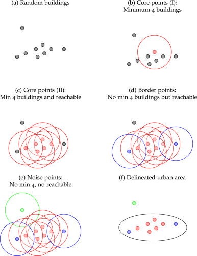
Once a set of buildings is identified as a cluster, this method draws its surrounding boundary using the α-shape algorithm Edelsbrunner et al. (1983), a widely used approach to delineate tight bounding boxes.

One of the key benefits of A-DBSCAN is that, because it relies on an ensemble approach that generates several candidate solutions, it allows us to explore to what extent boundaries are stable and clearcut or blurrier.

Dataset

Load dataset

We will be using the Berlin extract from Inside Airbnb. This is the same dataset used in the Scipy 2018 tutorial on Geospatial data analysis with Python.

To make the illustration run a bit speedier on any hardware, let us pick a random sample of 10% of the set; that is we’ll pick 2,000 properties at random.

For convenience, we convert into a GeoDataFrame where the geometries are built from the lon/lat columns in the original table.

berlin = gpd.read_file(r'..\map\berlin\berlin-listings.csv')
tab = berlin.sample(n=2000, random_state=1234)
db_ll = gpd.GeoDataFrame(tab,geometry=gpd.points_from_xy(tab.longitude, tab.latitude),crs={'init': 'epsg:4326'})
db_ll = db_ll.to_crs(epsg=5243)

The Code

By calling maps.cluster_a_dbscan,

adbs,lines = maps.cluster_a_dbscan(main_data, max_radius=500, figsize=[12,12])

This function requires the following parameters:

main_data (geodataframe): Data location and value
max_radius (int): maximum distance to look for neighbors from each location
figsize (tuple): figure size

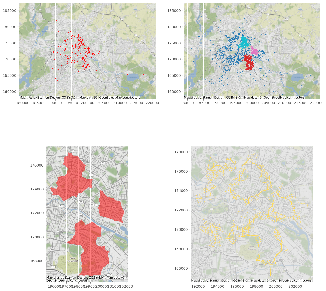
The result

drawing

The 1st image visualise our data.
The 2nd image displays each property colored based on its label assigned by a-dbscan algorithm.
The 3rd image displays some polygons that represent a tight boundary around all the points in a given cluster.
The 4th image displays extent boundaries and clearcut or blurrier.